Brief reflection: How would the content from the covered three lectures (18th, 21st, and 23rd August) relate to your project topic? How could it be put to use? Is there anything concrete in this direction that you would plan to research further, or that we should discuss together?
Schema.org is a semantic artefact supported by a community that includes Google, Microsoft, and Yahoo, and that organizes itself through the W3C. Explore schema.org from its online index. Additionally you could also load the ontology in TTL format into Protégé; however, schema.org should already be perfectly intelligible through its web-based documentation.
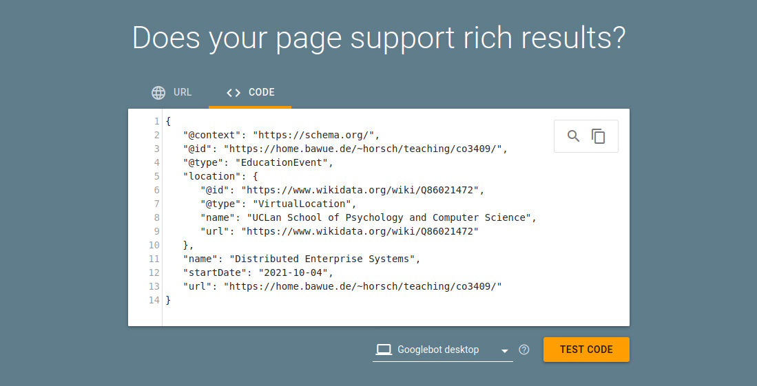
The HTML code of the module website (https://home.bawue.de/~horsch/teaching/dat121/index.html) contains a rudimentary schema.org based JSON-LD annotation. You can find it between the tags:
<script type="application/ld+json">
   …
</script>
How would you propose to modify and/or extend the annotation? Use the Google Rich Results Test to make sure that your revised annotation is processed by Google correctly.
Take the annotation that you introduced/modified in problem 2 using JSON-LD and write up the same triples in TTL format. (Not all the triples from the JSON-LD annotation - only those that you newly introduced or where you made modifications.)
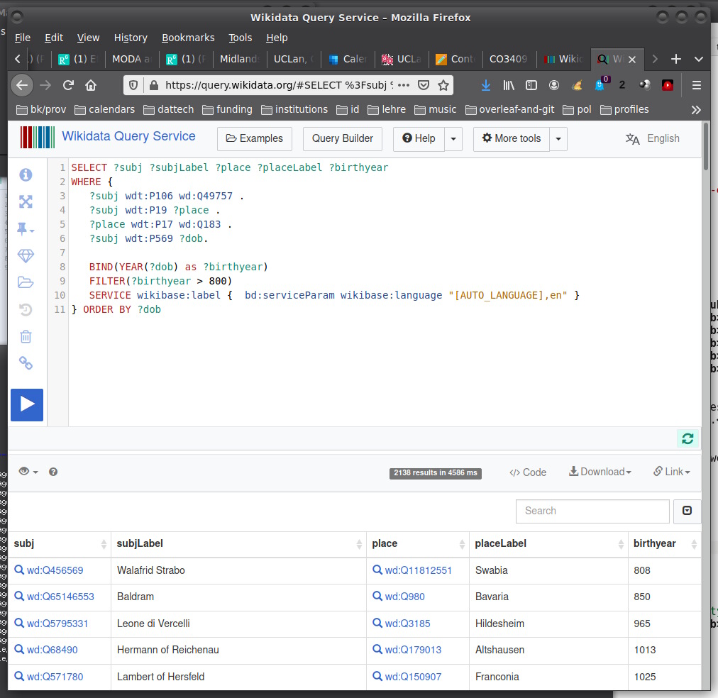
The Wikidata SPARQL end point is a good device for training yourself in the practical use of SPARQL. The documentation contains a long list of query examples. The IRIs used by Wikidata are resolvable, employing the following prefixes:
@prefix wd: <https://wikidata.org/wiki/>
@prefix wdt: <https://wikidata.org/wiki/Property:>
Accordingly, consider the following query from the list of examples:
# Birth places of German poets
#
SELECT ?subj ?subjLabel ?place ?placeLabel ?birthyear
WHERE {
   ?subj wdt:P106 wd:Q49757 .
   ?subj wdt:P19 ?place .
   ?place wdt:P17 wd:Q183 .
   ?subj wdt:P569 ?dob.

   BIND(YEAR(?dob) as ?birthyear)
   FILTER(?birthyear > 800)
   SERVICE wikibase:label {  bd:serviceParam wikibase:language "[AUTO_LANGUAGE],en" }
} ORDER BY ?dob
For example, in the first triple, wdt:P106 expands to https://wikidata.org/wiki/Property:P106, which is an object property labelled "occupation." The whole triple has the meaning "?subj has the occupation poet."
Practice formulating your own queries; for example, try asking for a table of Nobel laureates who are/were at some point affiliated with UiO. Repeat for NTNU. How many results do you obtain in each case, and do you agree with the response to your queries?
Apply regression using the statsmodels library to the data from the current table of Eliteserien. Based on these data, is there a significant correlation between the number of goals scored and the number of goals received? Is there a significant correlation between the number of draws and the goal difference? How about the number of draws and the square of the goal difference?
Consider the given data set consisting of 50 x-y pairs.
As an example time series, import and consider the development of the logarithm of the NOK:EUR exchange rate over the past year.
(a) Construct the residual (i.e., remainder) of the time series with respect to a zeroth-order (constant average value), first-order, and second-order regression. For each of the three residual curves, (b) compute the autocorrelation function, (c) use it to obtain at least a rough estimate of the decorrelation time, and (d) determine the interpolation error of the regression using Flyvbjerg-Pedersen block averaging.
The following glossary terms have been proposed for "Data and objects" (second lecture, 18th August): Knowledge base, knowledge graph (also: ABox), ontology (also: TBox), resource, triple. For "Regression basics," we had: Block averaging, decorrelation time (also: autocorrelation time), hypothesis, influence diagram, p value, regression analysis, residual quantity, supervised learning, uncertainty, validation and testing.
(submit through Canvas by end of 24th August 2023)